PWM 101: from Duty Cycle to Motor Control

Published onJune 22, 2023 Updated onJuly 16, 2023 Posted by Simona Di Domenico CategoryGeneral knowledge - Fundamentals

Introduction

Pulse Width Modulation is a powerful technique used in various applications in the world of electronics. It allows for the generation of square waves with a variable duty cycle, which can be used to control the amount of power delivered to a device.

In this article, we will delve into the theory behind PWM, explain the relationship between duty cycle and average, providing calculations, definitions, and diagrams to help you understand the concepts. Finally, we will explore some applications of PWM, such as LED dimming and motor control. By the end of this article, you will have a solid understanding of how PWM works and how it can be applied in practical situations.

Pulse width modulation

Pulse Width Modulation (often abbreviated as PWM) is a unit capable of generating pulse waves, periodic waves that alternate exclusively between two states: high and low. While readers may be familiar with the concept of square waves, it is important to highlight that those are particular types of pulse waves where the high and the low states last for the same amount of time.

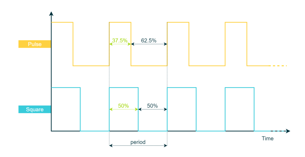
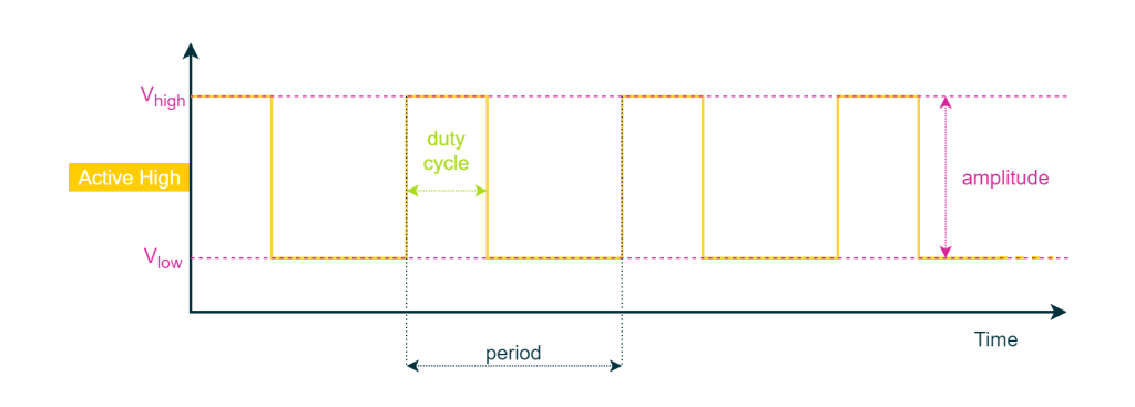
A pulse wave is a periodic signal that repeats itself at regular intervals. The time between successive repetitions of the waveform represents the period. Typically, the two states of a pulse wave are represented by different voltage levels, namely V_high and V_low.

Pulse wave: amplitude, period and levels

The unique characteristic of PWM is its capacity to adjust the width of the pulses, modifying the time duration of the ON and OFF states of the signal. Within a PWM signal, the ratio of the ON time to the total time (ON plus OFF) can be adjusted: this ratio is known as the Duty Cycle.

Initially designed for digital modulation, PWM was developed as a means of encoding information through the duty cycle of a square wave. However, its present-day application has shifted from information encoding to becoming the foundation of control systems, primarily employed for regulating the power delivered to a load.

Consequently, microcontrollers now frequently incorporate dedicated peripherals for generating PWM signals, making them prevalent in applications requiring system control. In many cases, microcontrollers can generate PWM signals purely in hardware, minimizing the need for software intervention. Software is required during the initial setup and infrequent adjustments at a rate significantly lower than the PWM frequency.

The concept of active and idle

The two possible states of a PWM signal can be referred to as active and idle, without specifically denoting high or low voltage levels.

Devices operate according to either active high or active low logic. An active high device is responsive to a logical high signal, while an active low device works with a logical low signal. For instance, if an LED is connected to a GPIO so that it lights up when the GPIO voltage is high, this means the LED works in active high logic. In this case, we can identify V_high as the active state and V_low as the idle state.

Consequently, the active state describes the operational phase of the device, and the idle state refers to its non-operational phase. It is essential to note that this classification is independent of voltage levels. Hence, there are two distinct types of PWM: Active High and Active Low, distinguished by the polarity of the signal.

Voltage	Active High PWM	Active Low PWM
V_high	active	idle
V_low	idle	active

Overview of voltage levels in Active High and Active Low PWM

As depicted in the table, in an Active High PWM, the active state is represented by V_high, while V_low represents the idle state. Conversely, for Active Low PWM, this is reversed (V_low is active, V_high is idle).

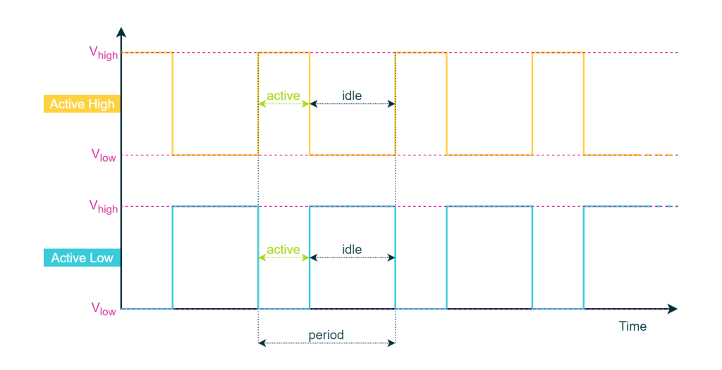
Active High and Active Low PWM with the same duty cycle

The image above displays active high and low PWM with identical duty cycles. From here and out, for the sake of maintaining generality, we will refer to the states as active and idle, rather than focusing on voltage levels.

Period and duty cycle

The period of a pulse wave is defined as the sum of the active time and the idle time. It represents the duration of one complete cycle:

$T = t_{active} + t_{idle}$

The frequency of the signal is defined as:

$f = \frac{1}{T}$

The duty cycle is the ratio between the active time and the period:

$D = \frac{t_{active}}{T}= \frac{t_{active}}{t_{active} + t_{idle}}$

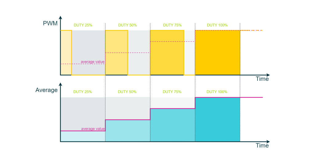
In general, in a PWM the period is kept constant while the share between active and idle states is changed over time. This represents a change in the duty cycle that is often expressed as a percentage. For instance, a 50% duty cycle implies an equal share between active and idle states (square wave). Extreme cases involve a duty cycle of 100%, meaning the signal remains active throughout the cycle, and 0%, indicating an entirely idle signal.

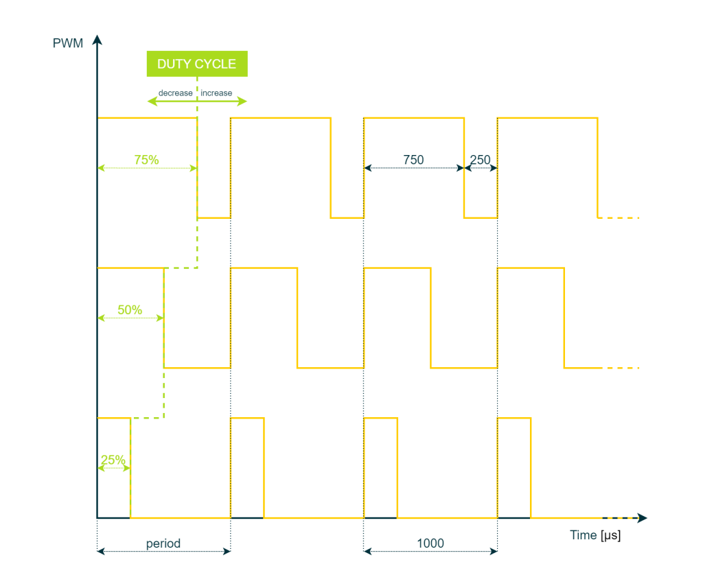
PWM waveforms with 75%, 50% and 25% duty cycle (Active High)

The image above shows the transition point between the active and idle states. The arrow direction signifies how this point can be shifted either to increase or decrease the duty cycle.

In this example, we have a PWM signal with a frequency of 1 kHz (or a period of 1 millisecond). In this case, a duty cycle of 75% means that the signal remains active for 750 microseconds and idle for the remaining 250 microseconds within a single period.

Relationship between Duty Cycle and Mean Value

The key feature of the PWM is the relationship between its duty cycle and its mean value. To understand better this relationship, let us consider an active high PWM with V_low equal to 0. We derived the complete equation step by step in the appendix. However, in this particular case, the mean value of the PWM signal is:

$\bar{x}(t)=D\cdot{V_{high}}$

We can notice that the average is proportional to the duty cycle and this means that by adjusting the duty cycle we can achieve the desired mean value. If the load is purely resistive, the current will be constant during the active state and null during the idle state. Therefore, acting on the duty cycle, we are effectively managing the amount of power delivered to the load. To some extent, this is true also with non-resistive loads. In this case, the equation, still a function of the duty cycle, would be a bit more complex.

The open question remains: how to extract the mean value of the PWM in electronics? This can be easily done by introducing a low-pass filter following the PWM signal generator. For instance, applying a low-pass filter with an extremely low cut-off frequency to an AC signal yields a DC signal that is the signal average value.

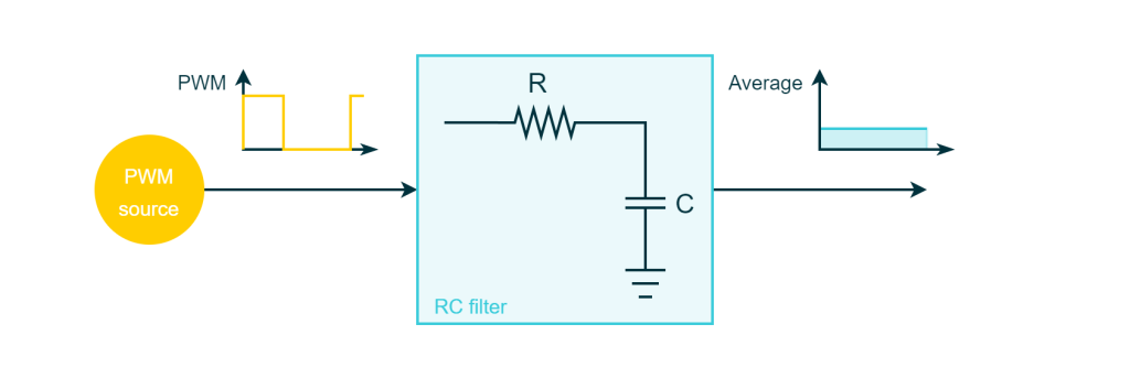
The block diagram below demonstrates a system composed of a PWM source and a low-pass filter. The PWM source generates the PWM signal, serving as the input for the low-pass filter. The filter output corresponds to the PWM signal average value.

Block diagram illustrating the PWM signal generator and low-pass filter

A common implementation of a low-pass filter is an RC filter, composed of a resistor and a capacitor. The input of the filter is the voltage provided to the RC branch and the output is the voltage on the capacitor (refer to RC circuit for more details).

Examples

The next section will delve into some examples of how to use a PWM signal in different scenarios. We will explore LED dimming, where the PWM signal and a low-pass filter manage LED brightness, and motor control, where the PWM allows to regulate the speed of a DC engine.

LED dimming

One of the most common applications of PWM in combination with low-pass filters is LED dimming. LEDs are widely used in lighting and display applications, and dimming them allows for better control of the brightness and color temperature. In this application, the human eye acts as a biological low-pass filter, smoothing out the PWM signal and making the LED appear dimmer.

The following block diagram extends the theoretical block diagram of the previous section. It consists of three blocks: the PWM source, the LED, and the human eye. The PWM source generates a voltage signal with a PWM waveform. The LED receives as input the PWM voltage signal and converts it into a corresponding PWM light signal (see A complete overview of LEDs for more details), resulting in a PWM light signal. This signal is then perceived by the human eye, which acts as a “biological filter”.

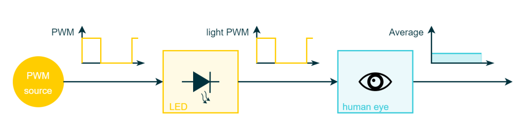
The cut-off frequency of the human eye refers to the highest frequency at which the eye can no longer perceive flickering or changes in light intensity. It depends on factors such as age and ambient lighting conditions and typically ranges from around 50 to 90 Hz.

If the frequency of the LED is higher than 90 Hz, the brain will perceive only the average value of light. However, if the frequency value is not high enough we will perceive flickering. A nice side note is that the old CRT screens were operating at a refresh rate of 60 Hz. This frequency is borderline and even if your eye doesn’t perceive the flickering, the brain does, which could cause headaches. So if you don’t want to hurt your final user, it would be better to dim a LED with a frequency of 100 Hz or more.

In conclusion, your visual system behaves as a low-pass filter and the brightness of light that you perceive is proportional to the duty cycle. In addition to traditional monochromatic LEDs, there are also RGB LEDs that contain multiple junctions, each emitting a different primary color: red, green, and blue. By controlling the brightness of each of these primary colors, it is possible to create any color in the visible spectrum.

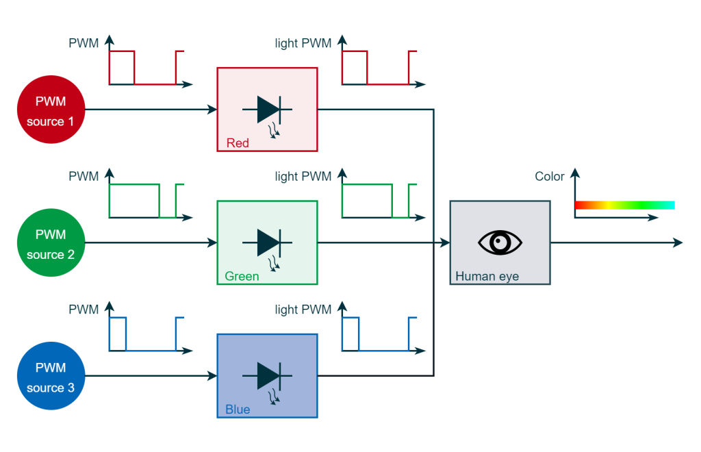
By varying the duty cycle of each color channel, the perceived color of the LED can be changed. For example, to create a yellow color, the red and green channels would be turned on while the blue channel would be turned off.

Motor control

Motors are substantially inductors and this makes them an interesting case for PWM control. By modulating the PWM signal, you essentially determine the amount of power transmitted to the load, which is directly proportional to voltage (V), current (I), and the duty cycle (D).

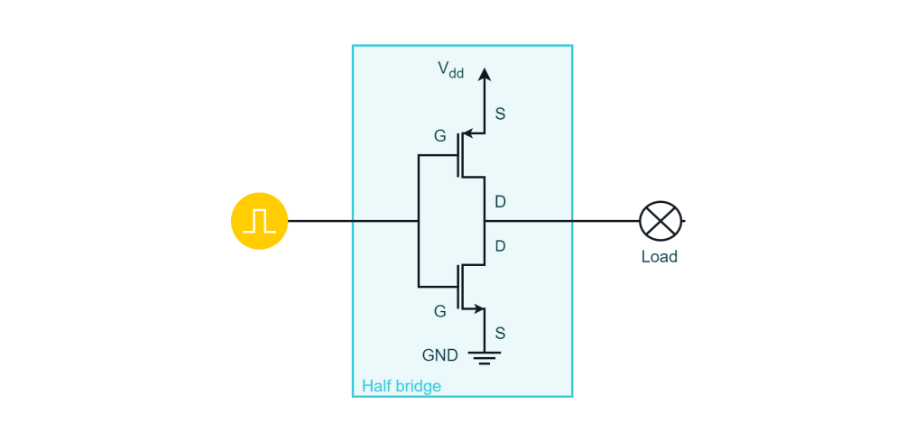
The picture above shows the configuration called a half-bridge, where power is transmitted in one direction. This setup uses high and low side switches operating in a complementary mode: one switch opens when the other closes, and vice versa. The high side switch is driven by the PWM signal, while the low side is driven by the negation of this signal.

By choosing the PWM duty cycle we determine the amount of current channeled from the supply to the engine, and ultimately, the amount of power delivered to the load. In this context, the current can flow only in one direction, thereby fixing the rotation direction of the engine. It is important to highlight the absence of a low-pass filter, as the motor, behaving like an inductor, acts as our low-pass filter.

A limitation of this circuit is the inability to choose the current direction. However, introducing a second half-bridge on the opposite side of the motor can overcome this issue.

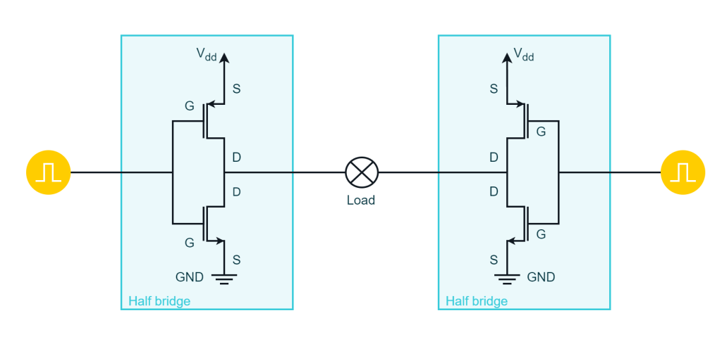
This circuit is known as Full Bridge or H-bridge due to its shape. In this case, the load is connected at both ends to two half bridges. Each bridge has separate PWM signals. If the left half-bridge operates at a variable duty cycle and the right bridge operates at a 0% duty cycle, we obtain the previous scenario where the duty cycle controlled the current entering the motor positive pole. Conversely, if the left half-bridge operates at a 0% duty cycle and the other operates at a variable duty cycle, the duty cycle controls a current that enters the motor negative pole, thereby reversing the rotation direction.

Conclusion

In summary, Pulse Width Modulation (PWM) is a key technique in electronics, controlling power delivery to a device by manipulating the duty cycle of square waves. This control over the duty cycle directly impacts the average value of the PWM signal. PWM demonstrates its versatility in LED dimming and motor control. From adjusting LED brightness and colors to managing motor control systems, PWM precise control solidifies its essential role in electronics.

Appendix A: Calculating the Average of a PWM Signal

In this appendix, we will see how to calculate the average of a PWM signal.

To determine the average value of a PWM signal, we can begin with its definition. The mean value for a periodic signal is obtained by integrating the signal over one period and dividing it by the period length:

$\bar{x}(t)=\frac{1}{T}\int_0^T x(t) \, \mathrm{d}t$

Considering that a PWM signal can be defined as:

$x(t) = \begin{cases} V_{high}, \;\;\text{if } 0 \leq x < DT. \\ V_{low}, \;\;\;\text{if } DT \leq x < T. \end{cases}$

the integral in the definition of mean value can be split into two parts:

$\bar{x}(t)=\frac{1}{T}\int_0^{DT} V_{high} \, \mathrm{d}t+\frac{1}{T}\int_{DT}^{T} V_{low} \, \mathrm{d}t$

Calculating the integral we obtain:

$\bar{x}(t)=D\cdot{V_{high}}+(1 - D)\cdot{V_{low}}$

The mean value of a PWM signal is given by:

$\bar{x}(t)=V_{low}+D\cdot{(V_{high}-V_{low})}$

The average value of a PWM signal is linearly dependent on the duty cycle. In simple terms, as the duty cycle increases, the average value of the signal also increases. Conversely, as the duty cycle decreases, the average value of the signal decreases as well.

In the special case where the low state is the reference ground (V_low = 0), the average value simplifies to: